Introduction to TensorFlow, TensorFlow Architecture with Example

What is TensorFlow

TensorFlow is a powerful open-source library developed by Google used for building machine learning and deep learning models. Both of which, are powerful ways computers can learn how inputs of a system are connected to outputs, just like how humans reason and learn. The model is first trained on some labeled data after which it can make predictions for unlabelled data.

TensorFlow was developed by a team of programmers and researchers on the Google Brain Team – a team under the umbrella of Google’s Machine Intelligence research organization. The team built TensorFlow to improve machine learning and deep learning (neural networks) methodologies.

Since then, TensorFlow has grown to be one of the most popular deep learning libraries, if not the most popular. TensorFlow is a great library for building huge projects with big data especially as neural networks perform better with big data. TensorFlow is used by Google, Apple, Samsung, NVIDIA, and many other big companies to build AI-powered systems such as recommendation, image captioning, text auto-completion, search engines, chatbots, etc. 

On YouTube, for instance, Google uses the very large dataset at their disposal to recommend tailor-suited videos to you. This is done by developing neural networks with TensorFlow to link videos with similar features (called content-based filtering) and users with similar preferences (called collaborative filtering). 

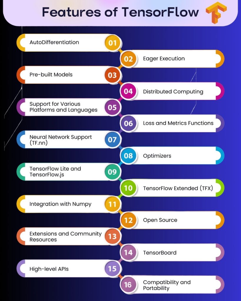
TensorFlow has some key features that make it popular. Let’s list out some of them. 

• Works efficiently for operations involving multi-dimensional vectors: The ‘tensor’ in TensorFlow is because it works with tensors – a mathematical representation of vectors or arrays, with respect to a vector space.
• High scalability: TensorFlow was designed to scale well which is important as data keep on increasing exponentially. Google search engine, for instance, does not store all the data on the web. But it has powerful computers that can scrap data from virtually all websites in a matter of seconds. As websites keep on springing up, TensorFlow’s framework can handle the increasing data and workload. 
• TensorFlow can run on more than one CPUs or GPUs. The same code can be computed on the two frameworks and even mobile operating systems.
• Supports neural networks and machine learning algorithms: As mentioned earlier, TensorFlow can be used to connect deep neural networks to map data features to labels and make predictions.

TensorFlow was written in C++ but can be used in many other programming languages like Python, Java, and C++. It can be also used with APIs which makes it a lot easier to play around with. A popular API is that supports TensorFlow is Keras. There are APIS for C++, Java, Rust, and other programming languages as well that can be used with TensorFlow.

In this tutorial, we will give you a gentle introduction to TensorFlow and touch the basics. By the end of this tutorial, here’s what you’ll learn:

• What is TensorFlow?
• A brief history of TensorFlow
• Where can TensorFlow run
• Why TensorFlow is so popular
• The Structure of TensorFlow Programs
• TensorFlow APIs
• Explaining TensorFlow with Examples

A Brief History of TensorFlow

When researchers and programmers started creating AI-powered systems, machine learning algorithms such as Linear Regression, Logistic Regression, K-Means, Support Vector Machine, Random Forest, etc. were used to build machine learning models. But as data grew larger, these machine learning algorithms didn’t have impressive performance. Then, deep learning methodologies sprung up which relatively did better compare to the machine learning algorithms especially when dealing with big data. 

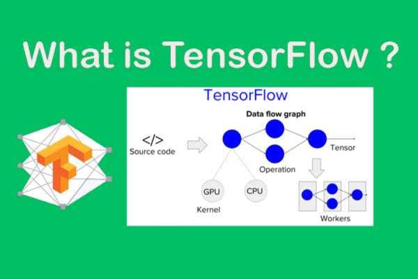
Before TensorFlow was developed, DistBelief was the primary deep learning framework for building deep neural nets. In February of 2017, the first version of TensorFlow was released by Google’s Brain team. The name ‘TensorFlow’ was coined from the word tensor which is a multidimensional array of numbers and the word ‘flow’ because you can visualize the flowchart of how different operations are carried out on input variables to return some output. 

In March 2018, the maiden version of tensorflow.js was officially announced. Tensorflow.js allows the building of machine learning models with JavaScript,. In January 2019, TensorFlow 2.0 was announced and was publicly made available in September that same year. TensorFlow 2.0 as since gained wide popularity especially as it incorporates a high-level API, Keras. 

Where can TensorFlow Run

To understand the requirements for TensorFlow usability in any device, we will split the software and hardware requirements into two phases. 

First is the development phase. In this phase, you train the model on some datasets. The trained model can be saved or reused for a different dataset or in a different machine entirely. It is advised to carry out the training process on a PC, rather than a mobile device anyway. Note that the training process can be done on more than one machine. This is particularly useful when you have a large dataset but not a single powerful machine. 

The second phase is the inference phase. After training the model, you need to run the model on new data to make predictions/inference. In this phase, you can run TensorFlow on a PC with Linux OS, mac OC, or Windows OS. You could also run it on mobile devices with Android or iOS. Furthermore, you could run the model on web cloud services such as Google Cloud Platform (GCP), Amazon Web Services (AWS), and Microsoft Azure. 

TensorFlow models can be trained on computer’s CPUs or GPUs. GPUs, however, tend to train the model faster as it is good in performing matrix and algebraic operations, which TensorFlow typically does. The fast computation of matrix and algebraic operations in TensorFlow can be attributed to the fact that it was written in C++. 

Why is TensorFlow so Popular

TensorFlow has grown to be the most widely used framework for building deep learning models for many reasons. First, of course, we would say because it is an open-source library – anybody and everybody can access and build on it. Also, TensorFlow allows for easy visualization of graphs and neural network connections with TensorBoard. Visualization of your neural nets is can come in handy when you want to debug your code. Moreso, this feature is not available in pandas or sci-kit learn library.

Furthermore, the fact that models can be easily trained on CPU and GPUs makes TensorFlow is accepted deep learning library. Not only that, you can train your model on multiple machines, which is great for large scale projects. In other words, TensorFlow is built to scale nicely and without hassle. 

TensorFlow also has a large pool of develops and by extension community who work round the clock to ensure the library is constantly being improved upon. 

The Architecture of TensorFlow

A TensorFlow program can be classified into two major structures, they are 

• The computational graph and
• The session. 

In the computational graph phase, the graph of hoe nodes combines using various operations is created. This is the stage where the dataset is preprocessed and the model is trained with the data. With TensorBoard, the computational graph can be seen 

In this phase, the computation graph is executed or run to produce some results. 

The library is called TensorFlow because it shows the flow chat of variables manipulated according to some rules to return some output. The diagram below shows a simple flow graph 

a and b are called input tensors while c is the resultant tensor. Multiply is a node that indicates the kind of operation that should be done with a and b to output c. 

In general, the nodes in a TensorFlow flow chart indicate the kind of mathematical operation while the edges in the graph, (also called tensor) are the mathematical array of the data whether as input or output. 

TensorFlow APIs

TensorFlow allows the use of the Application Programming Interface popularly called APIs. APIs can be somewhat seen as an intermediary between two applications. In this case, TensorFlow and the user. They are used to make reading and writing machine learning programs easier. APIs in general can be classified into two, they are:

• Low-level APIs: Low-end APIs are quite powerful, although sophisticated to use. They allow total control of the program and your model so it requires advanced domain knowledge and programming dexterity. Low-level APIs are mostly used by researchers. An example of a low-level TensorFlow API is the TensorFlow Core. 
• High-level APIs: High-level APIs on the other hand are easier to interact with and learn that the low-level counterpart. TensorFlow high-level API is built on top of TensorFlow Core. They are great for tasks where a lot of repetition and different users are involved. An example of a high-level API is Keras.

Let’s now go ahead to example a TensorFlow program, with examples. 

TensorFlow with Examples

Let’s start by running a simple TensorFlow program that multiplies two variables. 

#import the necessary library
import tensorflow as tf

#create the computational graph
#define the variable a and b which are constants
a = tf.constant(2.0)
b = tf.constant(4.0)
#multiply the two variables and define it as output c
c = tf.multiply(a, b)

#run the session
with tf.Session() as sess:
    #define the ran session as output
    output = sess.run(c)
    #print the output
    print(f"The output for this session is {output}")

Output:

The output for this session is 8.0

Let’s take a moment to understand what the code does. 

Step 1: We would need to define the input variables which are constants in this case. There are other methods other than tf.constant() to define variables. We will talk about the other popular methods going forward. 

Step 2: Afterwards, we can go ahead to define the computation, which is the tf.multiply() methods. Step 1 and 2 are the creation of the computational graph. A computational graph is a sequence of operations in TensorFlow, which are arranged into a graph of nodes and edges.

Step 3: Finally, we execute the operation. This is done in TensorFlow using the tf.Session() class as a defined variable. When we invoke the tf.Session() class, we ask TensorFlow to run the operations in the created computational graph. This is done by using the run() method of the invoked tf.Session() class. 

We can also define the variables as a list of numbers and carry out mathematical operations. Let’s see this example where we multiply two matrices and add their result. 

#import the necessary library
import tensorflow as tf   

#create the computational graph
#define the variable a and b
a = tf.constant([1, 2, 3, 4], dtype=tf.float64)
b = tf.constant([3, -4, 1, 1], dtype=tf.float64)
c = tf.constant([3, 1, 9, 12], dtype=tf.float64)
#multiply the two variables and define it as output c
d = tf.multiply(a, b)
e = tf.multiply(a, c)
final = tf.add(d, e)

#run the session
with tf.Session() as sess:
    #define the ran session as output
    output = sess.run(final)
    #print the output
    print(f"The output for this session is {output}")

Output:

The output for this session is [ 6. -6. 30. 52.]

It is important to note that printing the nodes without running them does not return a numerical value but the defined computational graph. Let’s attempt to print only the defined 

#import the necessary library
import tensorflow as tf

#create the computational graph
#define the variable a and b
a = tf.constant([1, 2, 3, 4], dtype=tf.float64)
b = tf.constant([3, -4, 1, 1], dtype=tf.float64)
c = tf.constant([3, 1, 9, 12], dtype=tf.float64)
#multiply the two variables and define it as output c
d = tf.multiply(a, b)
e = tf.multiply(a, c)
final = tf.add(d, e)

#print the outputs
print(d)
print(e)
print(final)

Output:

Tensor("Mul_8:0", shape=(4,), dtype=float64) 
Tensor("Mul_9:0", shape=(4,), dtype=float64) 
Tensor("Add_1:0", shape=(4,), dtype=float64)

As you can see from the output, the operations where not done on the variables because we didn’t run the computational graph. Remember that to run a session, you begin by instantiating the Session() class. Then you use the run() method to run the operations. Once you are done with a session, it is good practice to close it. You can do this using the close method. In our example, we would run:

sess.close()

Is TensorFlow Similar to NumPy?

If you have used NumPy before, you’d realize that tensors in TensorFlow are similar to NumPy n-dimensional arrays. TensorFlow can be used to do the basic NumPy operations and even more. To appreciate the similarity, let’s create a matrix using NumPy and TensorFlow. We would start with NumPy. 

#import the numpy library
import numpy as np

#define the matrices
matrix_a = np.arange(10)
matrix_b = matrix_a.reshape((5, 2))
matrix_c = matrix_b.sum(axis=0)
matrix_d = np.identity(4)

#print the matrices
print('Matrix A:', matrix_a)
print('Matrix B:', matrix_b)
print('Matrix C:', matrix_c)
print('Matrix D:', matrix_d)

Output:

Matrix A: [0 1 2 3 4 5 6 7 8 9] 
Matrix B: [[0 1] [2 3] [4 5] [6 7] [8 9]] 
Matrix C: [20 25] 
Matrix D: [[1. 0. 0. 0.] [0. 1. 0. 0.] [0. 0. 1. 0.] [0. 0. 0. 1.]]

Now, let’s do this same operation with TensorFlow

#import the tensorflow library
import tensorflow as tf

#instantiate the Session class
sess = tf.Session()

#define the matrices
matrix_a = tf.range(10)
matrix_b = tf.reshape(matrix_a, shape=(5, 2))
matrix_c = tf.reduce_sum(matrix_b, reduction_indices=[0])
matrix_d = tf.eye(5, 5)

#print the matrices
print('Matrix A:', sess.run(matrix_a))
print('Matrix B:', sess.run(matrix_b))
print('Matrix C:', sess.run(matrix_c))
print('Matrix D:', sess.run(matrix_d))

Output:

Matrix A: [0 1 2 3 4 5 6 7 8 9] 
Matrix B: [[0 1] [2 3] [4 5] [6 7] [8 9]] 
Matrix C: [20 25] 
Matrix D: [[1. 0. 0. 0. 0.] [0. 1. 0. 0. 0.] [0. 0. 1. 0. 0.] [0. 0. 0. 1. 0.] [0. 0. 0. 0. 1.]]

Notice they both produced the same result. 

Lets now talk about placeholders and variables. 

Placeholders

A placeholder is used to define an external input when creating a computational graph. When using a placeholder, you define the name of the variables where it’s the values will be stored, alongside its data type. You however do not provide the values for the placeholder at the point of creating the placeholder. The values are created when the graph is run in a session. 

The values of the placeholders are defined using the feed_dict argument of the run method. 

Let’s take an example. 

#import the tensorflow library
import tensorflow as tf
#define the placeholders
ph_1 = tf.placeholder(name='ph_1', dtype=tf.float64)
ph_2 = tf.placeholder(name='ph_2', dtype=tf.float64)

#define the operation
output_node = tf.multiply(ph_1, ph_2, name='output_node')

#define the session
with tf.Session() as sess:
    #run the session
    final_result = sess.run(output_node, feed_dict={
        ph_1: [-1, 2, 9],
        ph_2: [-3, -6, -1]
    })
    #print the result
    print(f"The final result is: {final_result}")

Output:

The final result is: [ 3. -12. -9.]

Let’s understand the above code line by line

Step 1:

ph_1 = tf.placeholder(name='ph_1', dtype=tf.float64)
ph_2 = tf.placeholder(name='ph_2', dtype=tf.float64)

When you define a placeholder, you do not define the values yet but the name and data type. For the example above, we called the placeholders ph_1 and ph_2, with a float64 dtype. 

Generally speaking, the placeholder takes in 3 parameters, the dtype, shape, and name. However, the dtype and name are optional parameters, i.e. the placeholder would still be created without them being explicitly defined. 

Step 2:

output_node = tf.multiply(ph_1, ph_2, name='output_node')

We need to specify the kind of operation that would be carried out on the input nodes. Here, we use the multiply() method to does the multiplication of the input nodes. 

Step 3:

with tf.Session() as sess:
    final_result = sess.run(output_node, feed_dict={
        ph_1: [-1, 2, 9],
        ph_2: [-3, -6, -1]
    })

This is the stage where you run the computational graph. The feed_dict argument of the run() method is where the values of the placeholders are defined, in a dictionary form. 

Variables 

Variables are used for storing and updating trainable parameters to an already defined computational graph. When defining a variable, the dtype and the initial value needs to be defined. The defined variable is initialized calling the global_variable_initializer() method. 

For example, we know that the equation of a straight line is y = mx + c where y and c are constant which can be updated for different lines. It becomes critical to use the Variable() class to define the m and c variable when running this in TensorFlow.  

Let’s see how to code this. 

#import the necessary libraries

#define the changeable variables 
m = tf.Variable([2], dtype=tf.float64)
c = tf.Variable([5], dtype=tf.float64)

#define the X values using placeholders
x = tf.placeholder(dtype=tf.float64, name='x')

#define the computation
y = m * x + c

#run the computation
with tf.Session() as sess:
    #initialize the global_variables_initializer()method
    initialize = tf.global_variables_initializer()
    sess.run(initialize)
    #define the final result
    final_result = sess.run(y, feed_dict={
        x: [1, 2, 3, 4, 5]
    })
    #print the final result
    print(f"The final result is: {final_result}")

Output:

The final result is: [ 7. 9. 11. 13. 15.]

Let’s understand what the above code does, line by line

Step 1: 

m = tf.Variable([2], dtype=tf.float64)
c = tf.Variable([5], dtype=tf.float64)
x = tf.placeholder(dtype=tf.float64, name='x')

We start by creating the computational graph. Here we used Variable() object to define the flexible variables while we used the placeholder() method to define the independent variable. Note that the values of the variable defined by the Variable() object were defined. Whereas the values of the variable defined by the placeholder() method were not defined.

Step 2:

y = m * x + c

We define the computation with which TensorFlow would run. Here, it was the equation of a straight-line y = mx + c. 

Step 3:

with tf.Session() as sess:
    #initialize the global_variables_initializer()method
    initialize = tf.global_variables_initializer()
    sess.run(initialize)
    #define the final result
    final_result = sess.run(y, feed_dict={
        x: [1, 2, 3, 4, 5]
    })
    #print the final result
    print(f"The final result is: {final_result}")

We then run the computation. First, we instantiate the Session() class and the global_varables_intializer() 

The 2 Methods to Load Data into TensorFlow

Data is the foundation of any machine learning system. It can be likened as the primary ingredient in preparing deep learning or machine learning model. That’s why you must know how to import data into TensorFlow. There are two basic ways of doing this. 

1. By loading the data in your computer memory: This is a way simpler method. It is as easy as creating an array or dataframe that stores your data. When you are dealing with relatively small data, say data less than 10GB, you can load it directly into your PC memory using method read_csv() from the pandas library. Or you could use the ‘with open’ statement to parse and append the file on your computer, line by line. 
2. By the TensorFlow data pipeline: You can also use TensorFlow built-in API to load data, carry out some operations, and feed the model very quickly. It is typically used for large datasets. If you have a dataset of 50GB for instance, and your PC has a memory of 8GB, certainly, your PC won’t be able to handle the data. This is what loading data with the TensorFlow pipeline comes in handy. 

Making use of a TensorFlow Architecture pipeline allows you to load large data in batches and across different CPUs. 

Now we can wrap up. We have discussed a lot of things in this tutorial but here are some of the key learning. 

• We said that TensorFlow is a popular and powerful deep learning library for building machine learning and deep learning models. 
• The reason for the popularity in TensorFlow is because it can run on a wide range of devices and operating systems without hassles. Furthermore, your project can scale easily with TensorFlow.
• We went on to see examples of how to carry out computations with TensorFlow. They can be done in two basic steps: create your computational graph and then run the computational graph on a session.